Descriptive geometry
Example
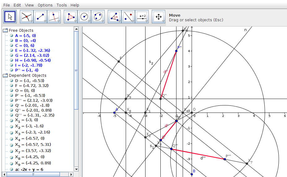
This is an example taught in the subject "descriptive geometry" (Darstellende Geometrie) at Austrian high schools and in specific engineering studies.
The problem is: Given a plane <math>\epsilon</math> by the traces <math>s_1, s_2</math> and a point <math>P</math> on <math>\epsilon</math> by projection by <math>P^{\prime\prime}</math>,
find a point <math>Q</math> with projection <math>Q^\prime</math> in top view and projection <math>Q^{\prime\prime}</math> in front view sucht that <math>Q</math> is on
the line of steepest descent on <math>\epsilon</math> in a distance of <math>3 {\it units}</math> below <math>P</math>.
Construction
The following construction has <math>A, B, C</math> as free points defining the plain <math>\epsilon</math> by the traces <math>s_1, s_2</math> and <math>P^{\prime\prime}</math> as free point. The other free points <math>E, G, H, I</math> are caused by colouring of the resulting lines <math>d^\prime, d^{\prime\prime}, d^{\prime\prime\prime}</math>.
Notation
For a readable description of the construction we propose the following notation
| <math>A^\prime, B^{\prime\prime}, P^{\prime\prime},X_1,X_2</math> | points in the plane (TODO make consistent using <math\prime</math> in construction) | ||
| <math>P</math> | point in the 3-dim. space with projections <math>(P^{\prime},P^{\prime\prime})</math> | ||
| <math>s_1,s_2,n</math> | straight lines | ||
| <math>\overline{l\,}</math> | length | ||
| A^\prime B^\prime|</math> | distance between point <math>A^\prime </math> and <math> B^\prime</math> on the plane | ||
| <math> | A B | </math> | distance between point <math>A </math> and <math> B</math> in space |
| <math>\overline{A B}</math> | the line through points <math>A, B</math> | ||
| <math>P \bot n</math> | the line through point <math>P</math> perpendicular to line <math>n</math> | ||
| <math>P | n</math> | the line through point <math>P</math> parallel to line <math>n</math> | |
| <math>n\vdash X^\prime \overline{l\,} +</math> | the point on line <math>n</math> with distance <math>\overline{l\,}</math> from point <math>X^\prime</math> in positive <math>+</math>orientation | ||
| <math>a \cap b</math> | the point intersecting lines <math>a</math> and <math>b</math> |
Program
Using these description we give a program below; the program takes the names <math>s_1,s_2, P^{\prime\prime}, \overline{d\,}</math> as arguments together with the respective coordinates and values. The names as arguments are useful for re-using the program as <math>{\it SubProblem}</math>.
The method names the horizontal axis <math>x</math>, the vertical axis <math>y</math> and creates an edge view of plane <math>\epsilon</math> in point <math>P^\prime</math> by <math>{\it SubProblem}({\it Geo},[{\it make},{\it proj}])</math>, which takes trace <math>s_1</math> and <math>P^\prime]</math> as arguments, constructs auxiliary view <math>n</math> and returnes the projection <math>p</math> (in the construction right bottom containing <math>P^{\prime\prime\prime}, Q^{\prime\prime\prime}</math>):
01  Program fallLinie <math>s_1(A(-5,0), B(0,-4))\;\;s_2(A(-5,0), C(0,6))\;\;P^{\prime\prime}(-1,5)</math>
      <math>(\overline{d\,}=3)</math> =
02    let <math>X_1 = {\it Take}\;x \cap \overline{P^{\prime\prime}B};</math>
03        <math>X_2 = {\it Take}\;X_1 || y;</math>
04        <math>P^\prime = {\it Take}\;\overline{X_2 O} \cap (P^{\prime\prime}|| y);</math>
05        <math>p = {\it SubProblem}({\it Geo},[{\it make},{\it proj}],[{\it make},{\it proj}])\;\;[s_1, P^\prime]</math>
06        <math>P^{\prime\prime\prime} = {\it Take}\;(P^\prime \bot n)\cap p ;</math>
07        <math>Q^{\prime\prime\prime} = {\it Take}\;p\vdash P^{\prime\prime\prime}\overline{d\,}- ;</math>
08        <math>Q^\prime = {\it Take}\;(Q^{\prime\prime\prime}\bot n)\cup n ;</math>
09        <math>X_8 = {\it Take}\;(Q^{\prime\prime\prime}\bot n)\cap x ;</math>
10        <math>X_9 = {\it Take}\;s_2\cap (X_8\bot x) ;</math>
11        <math>Q^{\prime\prime} = {\it Take}\;(X_9||x)\cap (Q^\prime\bot x) ;</math>
12    in <math>Q(Q^\prime,Q^{\prime\prime}) </math>
The tactics propagating the construction are Take and Subproblem.
Euqivalence of constructions
The program above shows a nice example for equivalences of constructions probably not yet accompished by ATP:
In lines 02..04 for point <math>P</math> on plane <math>\epsilon</math> the projection <math>P^\prime</math> is constructed from the given projection <math>P^{\prime\prime}</math> by using another point already given on <math>\epsilon</math>, <math>C=O</math>.
In lines 09..11 for point <math>Q</math> on plane <math>\epsilon</math> the projection <math>Q^{\prime\prime}</math> is constructed from the given projection <math>Q^\prime</math> by using the traces of <math>\epsilon</math>.
Another possibility would be to pack the problem for finding the other projection into a <math>{\it SubProblem}</math>, which would have the same postcondition for all methods:
input:         plain <math>\epsilon(s_1,s_2)</math>, point <math>P</math> with projection <math>P^\prime</math>
precondition:  <math>P \in \epsilon(s_1,s_2)</math>, lots of non-degeneracy conditions
output:        point <math>P^{\prime\prime}</math>
postcondition: <math>P(P^\prime,P^{\prime\prime})</math>
The above specification has different formalizations for different ATP-methods (see another example for the Area method). Particularly challenging are the postconditions: The postcondition for the <math>{\it SubProblem}</math> in the above program could be
<math>\forall P.\;P\in\epsilon\Leftrightarrow P^{\prime\prime\prime}\in n</math>